Deriving the Normal Distribution

This is part of an ongoing series of posts to relearn statistics. I'll attempt to do this by tackling problems that spurred the advancement of statistical methods and techniques. These posts will generally be a bit corny and/or lame, but I do think it helps to have a story like this when tackling a tricky concept. Also I'd like to point out that sections 6,7, and 8 are essentially copied from a UC Santa Cruz lecture I found online. I found it to be an extremely helpful resource in writing this post. It took me quite a bit of time to work through it but it really illustrated the usefulness of the big-O technique. I did fill in some of the steps that the author skipped over so I do feel I made some minor additions that prove useful. The lecture can be found at: UC Santa Cruz lecture

1 Introduction

One of the core tools used in statistics is the normal distribution. Very early on in my high school classes we were taught what it is and how to use it. That's all well and good, but I've always wondered where normal distributions come from. It's not at all a trivial distribution, and it seems like something that would be very difficult to notice. In fact I think it would be impossible. Sure, someone could notice that certain data points tend to cluster around a mean, but the acual pdf for a normal curve is: $$ f(x) = \frac{1}{\sigma\sqrt{2\pi}}e^{\frac{-(x-\mu)^{2}}{2\sigma^{2}}} $$ it seems highly unlikely that someone was able to look at normally distributed data and work out the above equation. So how was it discovered? From what I can tell, a number of mathematicians had danced around the concept, but Abraham De Moivre seems to be the name most associated with its discovery. I thought it was quite funny to learn that he developed it while consulting for gamblers who wanted to know what the true odds were of different games of chance. I never would have guessed that one of the most important statistical tools today was developed over 300 years ago to help gamblers.

Rather than retell his story though, I'll be telling a similar one to help illustrate the process. Note that as we begin here, we will be using the binomial distribution as our starting point. I won't be deriving this, but anyone so inclined can check out the "Tools of the Trade" post which gives a little more detail about it.

2 A Gambler’s Lament

We are going to transport ourselves back to the early 1700s and pretend we are mathematicians looking to put our skills to use. Given our reputation, we’ve been contact by a local gambler that needs our help. He would like to start gambling on coin tosses, and he needs to know whether the payout he’s being offered is fair. Here is what he can tell you about the game:

A coin is flipped 100 times and you must guess it correctly 70 times or more
You win 1000 times your wager if you are successful
There is a 50% chance to win each coin flip

You know it’s going to be tough, but you do have enough information to calculate the odds of winning. Let’s get cracking.

3 Getting Down with Binomial Distributions

The only real tool you have at your disposal here is the binomial distribution. Let us define the number of successfully guessed coin flips as $S$. We now have the following: $$ P(S \geq 70) = \sum_{k=70}^{100}{{100 \choose k}} \left(\frac{1}{2} \right)^{k} \left(\frac{1}{2} \right)^{n-k} = \sum_{k=70}^{100}{{100 \choose k}} \left(\frac{1}{2} \right)^{n} $$ Well calculating the binomial coefficient looks like it's going to be a real pain, although we have a trick up our sleeve. Recall that: $$ {N \choose k} = \frac{n!}{k!(n-k)!} $$ We see that we can "work our way up" to any value we like as follows: $$ {N \choose k+1} = \frac{n!}{(k+1)!(n-(k+1))!} = \frac{n!}{(k)!(n-k)!}\cdot \frac{n-k}{k+1} = {N \choose k} \cdot \frac{n-k}{k+1} $$ Starting with the fact that ${N \choose 0} = {N \choose N} = 1$ it would only take 30 multiplications and divisions to calculate all the binomial coefficients required. You would also need to calculate $\frac{1}{2^{100}}$ but that only requires 8 clever multiplications (I encourage you to try and figure out how to do this, but we won't be doing it here). Anyway, it's going to be a pain but we can do this all and it won't take $too$ long. Doing all this "by hand" yields: $$ \sum_{k=70}^{100}{{100 \choose k}} \left(\frac{1}{2} \right)^{n} \approx 0.00004 = 0.004\% = 1 \; in \; 25,000 $$ Well well well. It looks as though the gamblers have been getting absolutely fleeced by these odds. Even though the payout sounded very high, the odds of you winning are unbelievably low. Armed with this knowledge we go back and tell the person who hired us the news. They pay us for our services, leave, and tell everyone they know about your math consulting. "This is great!" you think. It took a decent amount of time but wasn't too hard, just tedious. Hopefully you get more opportunities like this.

4 More Opportunities Like This

As word spreads around about your ability to calculate odds for games of chace, you are soon inundated with requests from all around by people seeking to know more about games of chance; however, they are all slightly different. They all differ in how many trials are performed, how many they are required to win, and the probability of winning an individual trial. There is a lot of money to be made consulting for these people, but the endless tedium of these calculations is starting to wear on you. "There must a better way" you think. Maybe there's a way you can approximate the curve using a different function? It might not be exact, but hopefully it will be close enough. Let's take a more generalized approach than we did above, and call our number of successful trials $W$. Let's assume we have $n$ trials, want to predict the likelihood of $k$ successes, and each trial has probability of success $p$. In other words: $$ P(W = k) ={n \choose k} p^{k}(1-p)^{n-k} \quad \quad [1] $$ Let's also not forget that we also know: $$ E(W) = \mu_{W} = np $$ $$ var(W) = \sigma_{W}^{2} = np(1-p) $$ The ${n \choose k}$ term is the most difficult part to calculate, so let's see if we can do something with that. Recall Stirling's Approximation (and yes, this formula does predate common use of the normal distribution) which says: $$ n! = \sqrt{2\pi n} \left(\frac{n}{e} \right)^{n} $$ Plugging this into equation [1] yields the following (messy) equation: $$ f_{n,p}(k) = {n \choose k} p^{k}(1-p)^{n-k} = \frac{ \sqrt{2\pi n} \left(\frac{n}{e} \right)^{n}}{ \sqrt{2\pi k} \left(\frac{k}{e} \right)^{k} \sqrt{2\pi (n-k)} \left(\frac{n-k}{e} \right)^{n-k}} \cdot p^{k}(1-p)^{n-k} $$ $$ = \sqrt{\frac{n}{2\pi k(n-k)}} \left( \frac{np}{k} \right)^{k}\left( \frac{n(1-p)}{n-k} \right)^{n - k} \quad \quad [2] $$ At first this doesn't look like [2] will be very helpful at all. It's not at all clear how this will be easier to compute than what we had before. Before we proceed, let's take a quick detour to define some useful tools.

5 A Useful Taylor Series

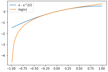
Generally speaking, a great tool to try when you need to deal with large exponents is the natural log function (denoted as $log(x)$ instead of the traditional $ln(x)$); however, it's not always the easiest function to use if we need to know exact values. Fret not though, as we can approximate it pretty well using a Taylor series. I'll skip the derivation, but note the following: $$ log(1+x) = x - \frac{x^{2}}{2} + \frac{x^{3}}{3} ... \; when \; -1 < x\leq1 $$ $$ x - \frac{x^{2}}{2} + O(x^{3}) \; as \; x \rightarrow 0 \quad \quad [3] $$ Seeing this you might have several questions: First off, why is it $log(1+x)$ instead of $log(x)$? Because $log(x)$ has a vertical asymptote at 0, it can be handy to shift it left one unit so we can center the Taylor Polynomial at 0. Second, is the two term approximation really that good? Here's what it looks like:

Figure 1: Taylor Series Approximation for log(x)

It looks like the approximation is pretty good in the positive numbers, but how about the negative? Isn't that a huge discrepancy? It might look like it, but we will eventually be exponentiating our numbers to return them to the "real world" in some sense. Here's what it looks like when we exponentiate the results:

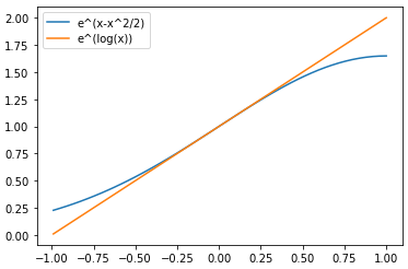
Figure 2: Exponentiation of Taylor Series Approximation of log(x) and actual log(x)

Now that looks MUCH better. Still not perfect at the endpoints, but certainly not as far off as it looked in the initial figure. Finally, what on Earth is the $O(x^{3})$ term in [3]? Admittedly this is still a new-to-me concept, but put as simply as possible I believe the general idea is "we don't care about subsequent terms since they'll all be really small". It allows us to focus on only a few terms and collect all subsequent terms in the "big O" term. (To be just a little more specific, we put a function in there which when multiplied by some constant value is larger than the error by truncating the remaining terms. It's imprecise, but gives a sense of how large the error will be and how it scales.) In this particular example, the exponents keep getting larger, but if $|x|<1$ then these terms get increasingly smaller. Anyway now that we've got a few new tools at our disposal, let's get back to some distributions.

6 Approximating the Exponent Terms

Before diving back into [2] above, let's define one last variable that will prove useful. In a lot of ways it can be helpful to think of how far we are from the mean of a given distribution. To that end, define $x$ to be: $$ x = k - np $$ We can immediately rewrite the above to get the following relationships: $$ k = np + x $$ $$ n - k = n(1-p) - x $$ Focusing on just the non square root terms of equation [2], taking some logs, and then substituting in $x$ we obtain the following: $$ \log \left( \left( \frac{np}{k} \right)^{k}\left( \frac{n(1-p)}{n-k} \right)^{n - k} \right) = -k \log\left(\frac{k}{np} \right) - (n-k) \log\left(\frac{n-k}{n(1-p)} \right) $$ $$ = -(np+x) \log\left(\frac{np+x}{np} \right) - (n(1-p)-x) \log\left(\frac{n(1-p)-x}{n(1-p)} \right) $$ $$ = -(np+x) \log\left(1 + \frac{x}{np} \right) - (n(1-p)-x) \log\left(1 - \frac{x}{n(1-p)} \right) $$ Now it feels like we're getting somewhere. We've been able to restate everything in terms of how far we are from the mean, and so long as $x$ is small compared to the quantities $np$ and $n(1-p)$ the arguments of our log function will fall within our radius of convergence. (This is one of the core assumptions we'll come back to in detail.) That's not all though, as all of the $\log$ terms can be hit with our Taylor series from above now because they're written in the form $\log(1+x)$. I'm going to skip over a lot of steps here, but applying our Taylor series from above and continuing the calculations from above gives: $$ \approx -(np+x)\left(\frac{x}{np} - \frac{1}{2}\left(\frac{x}{np}\right)^{2} + O\left(\frac{x^{3}}{n^{3}} \right) \right) -(n(1-p)-x)\left(\frac{-x}{n(1-p)} - \frac{1}{2}\left(\frac{x}{n(1-p)}\right)^{2} + O\left(\frac{x^{3}}{n^{3}} \right) \right) $$ $$ \approx -\left(x + \frac{x^{2}}{2np} + O\left(\frac{x^{3}}{n^{2}} \right) \right) - \left(-x + \frac{x^{2}}{2n(1-p)} + O\left(\frac{x^{3}}{n^{2}} \right) \right) $$ $$ = \frac{-x^{2}}{2np(1-p)} + O\left(\frac{x^{3}}{n^{2}} \right) $$ Now recalling our expressions for $\mu, \sigma^{2}$ and $x$, we can tidy up our equation with some back substitutions: $$ \log \left( \left( \frac{np}{k} \right)^{k}\left( \frac{n(1-p)}{n-k} \right)^{n - k} \right) = \frac{-(k-\mu)^{2}}{2\sigma^{2}} + O\left(\frac{x^{3}}{n^{2}} \right) $$ And now we can exponentiate both sides of the above expression and we obtain: $$ \left( \frac{np}{k} \right)^{k}\left( \frac{n(1-p)}{n-k} \right)^{n - k} \approx e^{ \frac{-(k-\mu)^{2}}{2\sigma^{2}}} \cdot e^{O\left(\frac{x^{3}}{n^{2}} \right)} \approx e^{ \frac{-(k-\mu)^{2}}{2\sigma^{2}}}\left(1+O\left(\frac{x^{3}}{n^{2}} \right) \right) \quad \quad [4] $$ Where the last simplification is made by using the first two terms of Taylor series approximation for $e^{x}$. Now this might start looking familiar to some of you, although we still have a pesky error term to deal with, as well as the square root term from [2]. Let's work our magic on that piece before dealing with these error terms.

7 Approximating the Square Root Term

Recall from above that the piece we would like to approximate is: $$ \sqrt{\frac{n}{2\pi k(n-k)}} \quad \quad [5] $$ Real quick before moving on I'd like to point out the following approximation: $$ f(x) = \frac{1}{\sqrt{x}} $$ $$ f(x+ \epsilon) \approx f(x)\left( 1 - \frac{\epsilon}{2x} \right), \; \epsilon << x $$ (This is simply approximating a nearby point using the value of the tangent line.) Now let's return to eqn. [5] and substitute in our x-values for the appropriate terms: $$ \sqrt{\frac{n}{2\pi (np+x)(n(1-p)-x)}} = \sqrt{\frac{1}{2\pi np(1-p) + O\left( x \right)}} $$ And because we'll generally expect $x$ to be quite a bit smaller than $n$, we can use our approximation above (as well as our previously covered expression for $\sigma^{2}$) and obtain the following: $$ f(2\pi n p (1-p) + O(x)) = \sqrt{\frac{1}{2\pi np(1-p) + O\left( x \right)}} \approx \frac{1}{\sigma \sqrt{2\pi}} \left(1- O\left( \frac{x}{n} \right) \right) \quad \quad [6] $$ Alright, now that we've managed to transform both pieces of [2], let's analyze our new distribution.

8 Your Favorite Distribution's Favorite Distribution

After all that, we can now combine [4] and [6] to rewrite expression [2] as follows: $$ f_{n,k} = f_{\mu,\sigma} \approx \frac{1}{\sigma \sqrt{2\pi}} e^{ \frac{-(k-\mu)^{2}}{2\sigma^{2}}}\left(1+O\left(\frac{x^{3}}{n^{2}} \right) \right) \left(1- O\left( \frac{x}{n} \right) \right) $$ Of course we still have to deal with those error terms, but the end is in sight. As I've alluded to earlier, our final assumption has to do with the size of $x$. Through all of our experience with binomial distributions, we've noticed that there's never been an observation that exceeds the mean by 5 standard deviations (note now we're talking about $\sigma$, not $\sigma^{2}$). It seems that no matter what our parameters are, even the most extreme observations seem to fall within a 5 standard deviation band around the mean, even as n grows quite large. (Of course they can exceed this, but we've been looking so long and haven't seen one it feels okay to ignore them.) Based on this assumption, we have: $$ |x| \leq 5\sqrt{np(1-p)} = O\left( \sqrt{n} \right) $$ Note that if we substitute this value for $x$ into both of the error terms above, we get: $$ \left(1+O\left(\frac{x^{3}}{n^{2}} \right) \right) = \left(1+O\left(\frac{1}{\sqrt{n}} \right) \right) $$ $$ \left(1-O\left(\frac{x}{n} \right) \right) = \left(1-O\left(\frac{1}{\sqrt{n}} \right) \right) $$ Which is great, because both terms will vanish as $n$ grows large! Excellent. Of course we don't have a set-in-stone definition of large, but this feels like a "we know it when we see it" situation. For $n$ sufficiently large, we have: $$ f_{\mu,\sigma}(k) \approx \frac{1}{\sigma \sqrt{2\pi}} e^{ \frac{-(k-\mu)^{2}}{2\sigma^{2}}} $$ And now for our variable $W$, we can calculate our probabilities like so: $$ P(a \leq W \leq b) = \frac{1}{\sigma \sqrt{2\pi}} \int_{a}^{b} e^{ \frac{-(k-\mu)^{2}}{2\sigma^{2}}} dk \quad \quad [7] $$ Is it time to pat ourselves on the back yet? Not quite, although I promise we're almost done.

9 But How do we Calculate That?

It begs the question, is [7] really more efficient to calculate than [2]? We can approximate [7] by taking very tiny Riemann sums, but that's going to be very labor intensive and require a lot of calculation for each problem. Was all this work for naught? Hopefully not, let's try one last thing. Let's define a new random variable $X = \frac{W - \mu}{\sigma}$. For each value $k$ that $W$ can take, we have a corresponding $x = \frac{k-\mu}{\sigma}$, and taking the derivative of that expression yields $\sigma dx = dk$. What happens if we plug this variable into[7]? We get: $$ P(a \leq W \leq b) = P(a \leq \sigma X + \mu \leq b) = P\left(\frac{a-\mu}{\sigma} \leq X \leq \frac{b-\mu}{\sigma} \right) $$ Which when plugged into [7] yields: $$ \frac{1}{\sigma \sqrt{2\pi}} \int_{\frac{a-\mu}{\sigma}}^{\frac{b-\mu}{\sigma}} e^{ \frac{-x^{2}}{2}} \sigma dx = \frac{1}{\sqrt{2\pi}} \int_{\frac{a-\mu}{\sigma}}^{\frac{b-\mu}{\sigma}} e^{ \frac{-x^{2}}{2}} dx \quad \quad [8] $$ And $finally$ we are finished. The integral in [8] no longer depends on our parameters (other than for determining the bounds of the integral). We only need to compute the values of the integral in equation [8] once, and then we can $always$ transform our binomial problems into this particular integral and get our answers quickly. Note that due to symmetry of the distribution and basic properties of probability, we only need to compute: $$ \frac{1}{\sqrt{2\pi}} \int_{0}^{c} e^{ \frac{-x^{2}}{2}} dx \quad \quad [9] $$ for $0 \leq c \leq 5$ incrementing $c$ by 0.01 and that should be enough to solve every problem you come across. Anything beyond this is so rare it's unlikely to ever happen during your lifetime in a simple game of chance, so there's no reason to know the exact probability.

10 Verifying That Our Approximation Is Good

Historically, people did calculate values of [9] by hand and stored them in reference tables, but we won't be doing that here (it's incredibly tedious). Let's take a brief moment just to check that our approximation accurately models the coin game above and get out of here. First let's check what the entire distribution looks like:

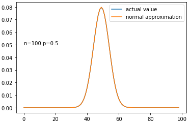
Figure 3: Comparison of Binomial Distribution and Normal Approximation

You can't even see both curves as they're directly on top of one another so I feel pretty good about the approximation. Let's quickly check what the actual and approximate values are for some particular values (and note that due to the nature of discrete vs. continuous values we must add 0.5 to the continuous value):

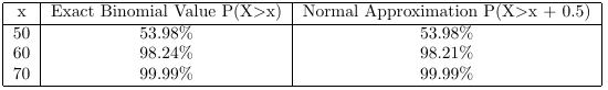
Figure 4: Table comparing actual and approximated values

A few thoughts: I always mess this sort of thing up, but I thought 50 would be the 50\% point. 50 is the mean, but 0$\leq$x$\leq$50 is actually 51 out of 101 buckets, so it's not surprising that it's over 50\%. Second, the approximation looks like it's very good for practical purposes. We're off by 0.03\% in the x=60 case, but you have to go out to the third and fourth decimal places to get a mismatch. Of course we shouldn't be lulled into a false sense of security. Our number of trials is large here so things "in the middle" are generally pretty good, but don't forget the derivation. If n is small our error terms aren't completely negligible (think back to the big-O terms proportional to $\frac{1}{\sqrt{n}}$). The approximation also becomes increasingly bad for tail events. Remember that we needed our deviation from the mean to be "small" in some sense, and if it's very large those higher order terms can't be ignored. Now I should clarify here that "bad" is a relative term. Our approximation of a tail event could be off by a factor of 1000, but when both events have a probability less that $10^{-10}$ it doesn't $really$ matter.

11 Wrapping Up

Thank you to all the reader(s) who made it this far. Not only was this post long and technical, but you had to put up with my lame story telling as well. I learned a ton researching this post and I'm excited to write a few more of these. The next two topics I'm interested in are the t-distribution and $\chi^{2}$ distribution. Both are extremely important in statistics but are even more confusing and arbitrary-seeming that the normal distribution. After those I think I think we should be ready to move on to some hypothesis testing and regressions.

I'd also like to bring attention to a topic that I found extremely interesting: The appearance of $\pi$ in the normal approximation and other formulas. I didn't go too in depth into Stirling's approximation here or mention the Wallis product, but the appearance of $\pi$ in all of them is a fascinating fact that shows an interesting (an unexpected relationship) between all of these ideas. In fact, I'd say over 75\% of my research on this post was on those three formulas and really trying to wrap my head around them. They were some of the earliest tools available to mathematicians trying to step from the discrete into the continuous world. To summarize: the Wallis product is really just a trig integral in disguise (which is how the $\pi$ term appears), Stirling's approximation gives us a continuous form of the factorial function that can be cleverly rewritten to look like the Wallis approximation (and gives a minor sense of where the $\pi$ term comes from), and the normal distribution is really just the continuous form of the binomial distirbution which we can derive using Stirling's approximation.

(Not that anyone asked, but the proof found in the "tricks of the trade" section of this statistics blog is excellent for showing the relationship between Stirling and Wallis, but deriving the Stirling formula is where things get a bit tricky. It seems impossible to side step the Euler-McLaurin formula and admittedly this is still a concept I'm learning how to use. It's extremely powerful and looks like something worth investigating more, but it's just taking me some time to wrap my head around it.)

Just want to give another shoutout to the lecture linked above too. I tried doing some of this on my own but it's clear I didn't have the tools necessary to do it.